Receiver module: Defining the receiver geometry
Receiver system
As described in the overview, the user must provide the geometric
definition of the tubular receiver and the mechanical and thermal
boundary conditions as part of the required package input.
The srlife.receiver module defines data structures for providing
this information and some simple methods for manipulating the data.
The python class srlife.receiver.Receiver provides the top level
interface and uses a hierarchy of objects to describe the receiver
geometry and boundary conditions. The figure below describes the structure.
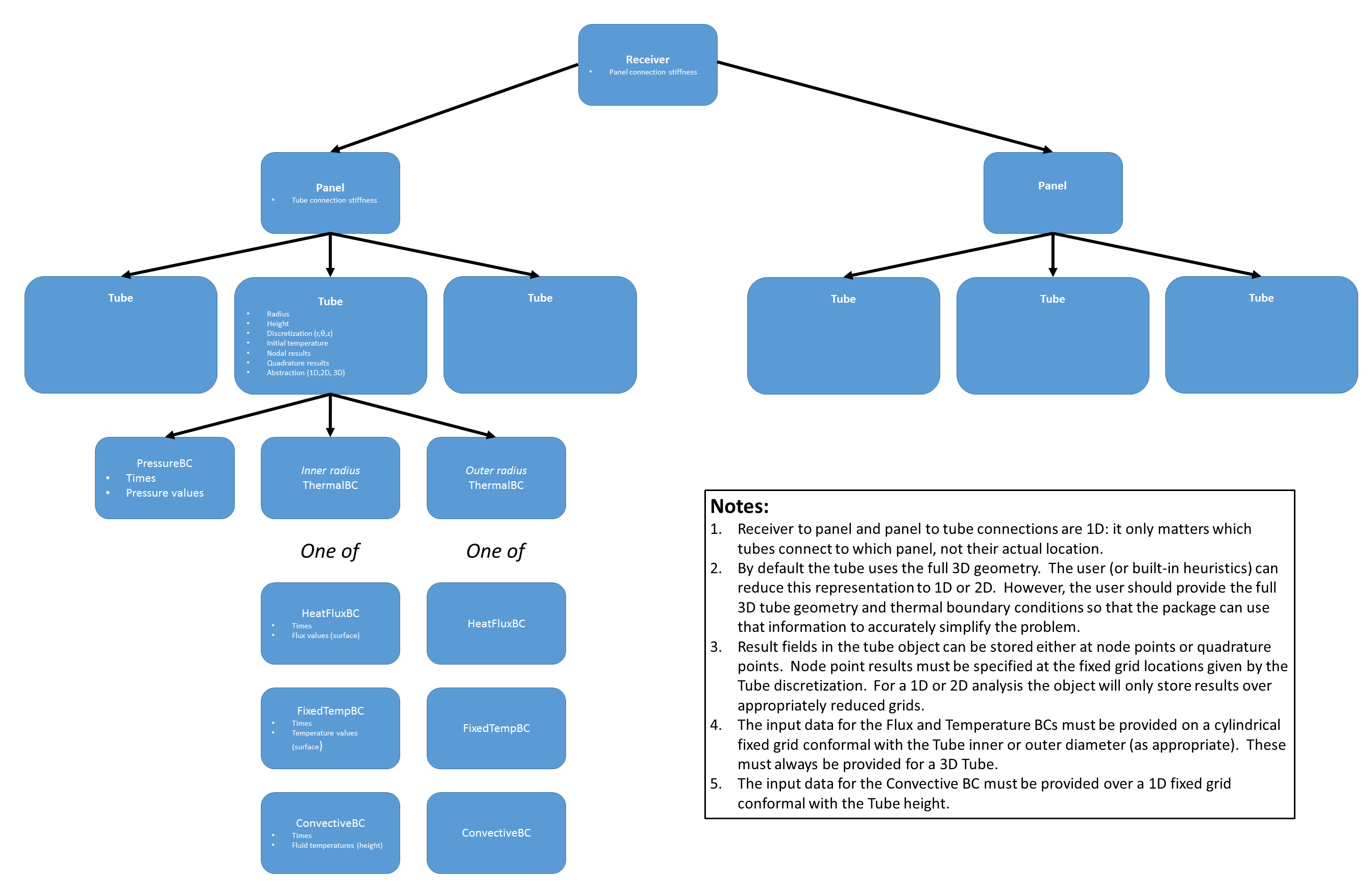
The overall data structure is hierarchical, descending from the single
srlife.receiver.Receiver object describing the entire receiver.
The receiver has one or more srlife.receiver.Panel objects
each of which have one ore more srlife.receiver.Tube objects.
Structurally, each tube in a panel is connected through its top-surface
displacement through a spring. Similarly, each panel is connected to the
other panels through a spring. The spring stiffness defines the type
of connection, options are:
A string “disconnect” meaning the spring has zero stiffness and the member floats freely, not connected to the result of the objects of its type.
A string “rigid” which means the object is rigidly connected to the others of its type with an infinitely-rigid spring.
A float giving the discrete spring stiffness.
The srlife.receiver.Receiver structure itself stores additional metadata:
The cycle period. Typically this will be 24 hours, but could be a reduced representation, for example cutting out a period of the hold in the cold nighttime condition.
The number of days (cycle repetitions) actually represented in the structural and thermal boundary conditions. This could, and almost always will be, not the full receiver life in days as the prescribed loads could represent a larger number of actual repetitions in service.
The Tube object holds basic geometric information describing a cylindrical tube, the tube discretization which is a fixed grid in cylindrical coordinates given by a fixed number of radial, circumferential, and axial subdivisions, the initial tube temperature, the discrete times at which the object stores boundary condition information and results, zero or more nodal results fields, zero or more quadrature result fields, an optional inner pressure boundary condition, an optional inner diameter thermal boundary condition, and an optional outer diameter thermal boundary condition. In addition, the tube carries a flag indicating whether the tube should be treated with a full 3D analysis or a reduced 2D or 1D analysis. For the reduced analysis the tube retains the height of the slice (2D and 1D) and the angle of the slice (1D), with respect to the full 3D cylindrical coordinate system.
The tube result and boundary condition times are a 1D array of time values, starting at zero. This array has length \(n_{time}\) and must be consistent for all the nodal results, quadrature results, pressure boundary conditions, and thermal boundary conditions.
Nodal results are stored on a fixed grid defined by an array of size
where \(n_{r}\) is the number of radial grid points, \(n_{\theta}\) is the number of circumferential grid points, and \(n_z\) is the number of axial grid points. A 2D representation leaves off the last axis and a 1D representation leaves off the last two axes.
The inner pressure boundary condition srlife.receiver.PressureBC holds a 1D array of pressures
defining the pressure at discrete times. The size of this 1D array
must be \(n_{time}\) and match the tube object.
The user has two options for outer diameter thermal boundary conditions:
Fixed flux boundary condition
srlife.receiver.HeatFluxBC.Fixed temperature boundary condition
srlife.receiver.FixedTempBC.
The data for the flux and temperature boundary conditions is an array of flux or temperature values of size
representing a fixed grid of points on either the tube inner or outer diameter. The user must provide the full 3D data.
Inner tube thermal BCs
By default, the inner boundary condition for each tube is a representation of heat transfer between the tubes and the working fluid. Two separate solvers are used to balance heat transfer between the tube and the fluid: a finite difference, 1D/2D/3D transient heat transfer solver for the solid temperatures and a 1D transient thermohydraulic solver for the fluid temperatures. The boundary conditions for the finite difference solver are the outside diameter boundary condition specified by the user for each tube (often the net incident flux) and convective heat transfer between the tube inner diameter and the fluid. The input conditions for the thermohydraulic solver are the flow rate and inlet temperature along each flow path in the receiver, given as a function of time throughout the user-provided load history. Heat then transfers along each flow path, with the fluid absorbing heat from each tube in the path.
These two solvers are coupled along the inner diameter of each tube. srlife solves for overall heat balance using Picard iteration on the heat transfered from the tube into the fluid (equal to the heat transfered out of the fluid and into each tube). This means that the solver starts with a guess at what this convective heat transfer will be, solves for the metal temperatures, calculates the convective heat transfer into the fluid, solves for the fluid temperatures, and iterates to solve again for the tube temperatures. This process repeats until both the fluid and tube temperatures no longer change.
The previous section discusses specifying the tube outer diameter boundary conditions, which, again, are often the next
incident flux directed at each tube in the receiver.
The model divides up the panels in the receiver into one or more flow paths. Fluid flows into the
first panel, through the panel, into the next connected panel, and so on until it reaches the panel outlet.
The user specifies which panels in the receiver are connected with a method of the srlife.receiver.Receiver
class
receiver.add_flowpath(panels, times, flow_rate, inlet_temp)
where the method takes as input a list of panels in the flow path, in the order the fluid flow through time, a numpy array of times throughout the loading history for which the flow_rate and inlet_temp arrays provide the corresponding inlet mass flow rates and inlet temperatures.
Each panel in the receiver must belong to one and only one flow path.
A model of a tubular panel receiver can explicitly represent fewer tubes than the actual number in each panel to
save computational cost. Because the structural damage and reliability models base the overall performance of
the receiver on the worst (most damaged/least reliable) tube, these models do not need any special modification to
accommodate models that use fewer than the full number of tubes to represent each panel. However, the
flow velocity through each tube depends on overall mass flow rate into a panel and the actual number of tubes
the flow divides into in that panel. Each srlife.receiver.Tube in the srlife.receiver.Receiver
has a multiplier property that the user can set to have the tube represent more than one tube in the actual panel
for the thermohydraulic calculation. For example, if there are 100 tubes in the actual panel and the user
represents only two tubes per panel in the actual thermal and structural model then this multiplier could be:
for tube in panel.tubes:
   tube.multiplier = 50
Defining the model
- The user can provide the required input data in two ways:
The Python objects
An HDF5 file
Both methods provide options for linking into external programs.
Python objects
Receiver geometry
The Receiver object contains panels and the interconnect spring stiffness between the panels.
- class srlife.receiver.Receiver(period, days, panel_stiffness)
Basic definition of the tubular receiver geometry.
A receiver is a collection of panels linked together by an elastic spring stiffness. This stiffness can be a real number, “rigid” or “disconnect”
Panels can be labeled by strings. By default the names are sequential numbers.
- In addition this object stores some required metadata:
The daily cycle period (which can be less than 24 hours if the analysis neglects some of the night period)
The number of days (see #1) explicitly represented in the analysis results.
- Parameters:
period (float) – single daily cycle period
days (int) – number of daily cycles explicitly represented
panel_stiffness (float or string) – panel stiffness (float) or “rigid” or “disconnect”
- add_flowpath(panels_in_path, times, mass_rate, inlet_temp, name=None)
Add a flow path to the receiver model
- Parameters:
panels_in_path (list) – list of panel names in the path
times (np.array) – time data
mass_rate (np.array) – mass flow rate data
inlet_temp (np.array) – inlet temperature data
name (Optional[str]) – optional flowpath name
- add_panel(panel, name=None)
Add a panel object to the receiver
- Parameters:
panel (Panel) – panel object
name (Optional[str]) – panel name, by default follows fixed scheme
- close(other)
Check to see if two objects are nearly equal.
Primarily used for testing
- Parameters:
other (Receiver) – the object to compare against
- Returns:
True if the receivers are similar.
- Return type:
bool
- classmethod load(fobj)
Load a Receiver from an HDF5 file
A full description of the HDF format is included in the module documentation
- Parameters:
fobj (string) – either a h5py file object or a filename
- Returns:
The constructed receiver object.
- Return type:
- property npanels
Number of panels in the receiver
- Returns:
Number of panels
- Return type:
int
- property ntubes
Shortcut for total number of tubes
- Returns:
Number of tubes in all panels
- Return type:
int
- save(fobj)
Save to an HDF5 file
This saves a Receiver object to the HDF5 format.
- Parameters:
fobj (str) – either a h5py file object or a filename
- set_paging(page)
Tell tubes to store results on or off disk
- Parameters:
page (bool) – if true, page results to disk
- property tubes
Shortcut iterator over all tubes
- Returns:
iterator over panels
- write_vtk(basename)
Write out the receiver as individual panels with names basename_panelname
The VTK format is mostly used for additional postprocessing. The VTK format cannot be used for input.
- Parameters:
basename (str) – base file name
The Panel object contains tubes and the interconnect spring stiffness between each tube in the panel
- class srlife.receiver.Panel(stiffness, ntubes_actual=None)
Basic definition of a panel in a tubular receiver.
A panel is a collection of Tube object linked together by an elastic spring stiffness. This stiffness can be a real number, a string “disconnect” or a string “rigid”
Tubes in the panel can be labeled by strings. By default the names are sequential numbers.
- Parameters:
stiffness – manifold spring stiffness
- add_tube(tube, name=None)
Add a tube object to the panel
- Parameters:
tube (Tube) – tube object
name (Optional[str]) – Tube name, defaults to fixed scheme.
- close(other)
Check to see if two objects are nearly equal.
Primarily used for testing
- Parameters:
other (Panel) – the object to compare against
- Returns:
true if the panels are sufficiently similar
- Return type:
bool
- classmethod load(fobj)
Load from an HDF5 file
- Parameters:
fobj (h5py.Group) – h5py group containing the panel
- property ntubes
Number of tubes in the panel
- Returns:
number of tubes in the panel
- Return type:
int
- property ntubes_actual
Number of actual tubes in the panel
- Returns:
number of tubes in the full panel
- Return type:
int
- save(fobj)
Save to an HDF5 file
- Parameters:
fobj (h5py.Group) – h5py group
- write_vtk(basename)
Write out the panels as individual tubes with names basename_tubename
- Parameters:
basename (string) – base file name
The Tube object contains the majority of the analysis information and results of the analysis. The structure holds the basic tube geometry, the tube discretization, described as intervals in a cylindrical coordinate system, and initial tube temperature, the thermal and mechanical boundary conditions, and result fields stored at discrete times and either at node points or quadrature points.
- class srlife.receiver.Tube(outer_radius, thickness, height, nr, nt, nz, T0=0.0, page=False, multiplier=1)
Geometry, boundary conditions, and results for a single tube.
The basic tube geometry is defined by an outer radius, thickness, and height.
Results are given at fixed times and on a regular polar grid defined by a number of r, theta, and z increments. The grid points are then deduced by linear subdivision in r between the outer radius and the outer radius - t, 0 to 2 pi, and 0 to the tube height.
Result fields are general and provided by a list of names. The receiver package uses the metal temperatures, stresses, mechanical strains, and inelastic strains.
Analysis results can be provided over the full 3D grid (default), a single 2D plane (identified by a height), or a single 1D line (identified by a height and a theta position)
Boundary conditions may be provided in two ways, either as fluid conditions or net heat fluxes. These are defined in the HeatFluxBC or ConvectionBC objects below.
- Parameters:
outer_radius (float) – tube outer radius
thickness (float) – tube thickness
height (float) – tube height
nr (int) – number of radial increments
nt (int) – number of circumferential increments
nz (int) – number of axial increments
T0 (Optional[float]) – initial temperature
page (Optional[bool]) – store results on disk if True
multiplier (Optional[int]) – number of tubes represented by this actual model, defaults to 1
- add_axial_results(name, data)
Add a result distributed over the tube height at nz points
- Parameters:
name (str) – results name
data (np.array) – data to store
- add_blank_axial_results(name)
Add a blank axial results field
- Parameters:
name (str) – name of field
- add_blank_quadrature_results(name, shape)
Add a blank quadrature point result field
- Parameters:
name (str) – parameter set name
shape (tuple) – required shape
- add_blank_results(name, shape)
Add a blank node point result field
- Parameters:
name (str) – parameter set name
shape (tuple) – required shape
- add_quadrature_results(name, data)
Add a result at the quadrature points
- Parameters:
name (str) – parameter set name
data (np.array) – actual results data
- add_results(name, data)
Add a node point result field
- Parameters:
name (str) – parameter set name
data (np.array) – actual results data
- close(other)
Check to see if two objects are nearly equal.
Primarily used for testing
- Parameters:
other (Tube) – the object to compare against
- Returns:
true if the tubes are similar
- Return type:
bool
- copy_results(other)
Copy the results fields from one tube to another
- Parameters:
other – other tube object
- property dim
Actual problem discretization
- Returns:
tuple giving the fixed grid discretization
- Return type:
tuple(int)
- element_surface_areas()
Calculate the element surface areas
- Returns:
np.array with each element area
- element_volumes()
Calculate the element volumes
- Returns:
np.array with each element volume
- classmethod load(fobj)
Load from an HDF5 file
- Parameters:
fobj (h5py.Group) – h5py to load from
- make_1D(height, angle)
Abstract the tube as 1D
Reduce to a 1D abstraction along a ray given by the provided height and angle.
- Parameters:
height (float) – the height of the ray
angle (float) – the angle, in radians
- make_2D(height)
Abstract the tube as 2D
Reduce to a 2D abstraction by slicing the tube at the indicated height
- Parameters:
height (float) – the height at which to slice
- property mesh
Calculate the problem mesh (should only be needed for I/O)
- Returns:
Results of np.meshgrid over the problem discretization
- property multiplier
Number of actual tubes represented by this model
- Returns:
tube multiplier
- Return type:
int
- property ndim
Number of problem dimensions
- Returns:
tube dimension
- Return type:
int
- property ntime
Number of time steps
- Returns:
number of time steps
- Return type:
int
- save(fobj)
Save to an HDF5 file
- Parameters:
fobj (h5py.Group) – h5py group to save to
- set_bc(bc, loc)
Set the inner or outer heat flux BC
- Parameters:
bc (ThermalBC) – boundary condition object
loc (string) – location – either “inner” or “outer” wall
- set_paging(page, i)
Set the value of the page parameter
- Parameters:
page – if true store results on disk
i – tube number to use
- set_pressure_bc(bc)
Set the pressure boundary condition
- Parameters:
bc (PressureBC) – boundary condition object
- set_times(times)
Set the times at which data is provided
All results arrays must provide data at these discrete times.
- Parameters:
times (np.array) – time values
- surface_elements()
Return an indication of which are surface elements and their normal vectors.
- Returns:
logical indexing array, True if on surface np.array of surface normals (zeros for solids)
- write_vtk(fname)
Write to a VTK file
The tube VTK files are only used for output and postprocessign
- Parameters:
fname (string) – base filename
Boundary conditions
The only mechanical boundary condition the user needs to specify is the Tube internal pressure.
- class srlife.receiver.PressureBC(times, data)
Stores information about the tube internal pressure
Simple class to store tube pressure, assumed to be constant in space and just vary with time.
- Parameters:
times (np.array) – times throughout load cycle
data (np.array) – pressure values
- close(other)
Test method for comparing BCs
- Parameters:
other (PressureBC) – other object
- Returns:
true if the objects are sufficiently similar
- Return type:
bool
- classmethod load(fobj)
Load from an HDF5 file
- Parameters:
fobj (h5py.Group) – h5py group to load from
- property ntime
Number of time steps
- Returns:
number of time steps in the pressure history definition
- Return type:
int
- pressure(t)
Return the pressure as a function of time
- Parameters:
t (float) – time
- Returns:
internal pressure at that time
- Return type:
float
- save(fobj)
Save to an HDF5 file
- Parameters:
fobj (h5py.Group) – h5py group to save to
Superclass handing HDF storage dispatch for thermal boundary conditions
- class srlife.receiver.ThermalBC
Superclass for thermal boundary conditions.
Currently just here to handle dispatch for HDF files
Thermal boundary conditions options are fixed flux (HeatFluxBC), fixed temperature (FixedTempBC), and convection (ConvectiveBC).
- class srlife.receiver.HeatFluxBC(radius, height, nt, nz, times, data)
A net heat flux on the radius of a tube. Positive is heat input, negative is heat output.
These conditions are defined on the surface of a tube at fixed times given by a radius and a height. The radius is not used in defining the BC but is used to ensure the BC is consistent with the Tube object.
The heat flux is given on a regular grid of theta, z points each defined but a number of increments. This grid need not agree with the Tube solid grid.
- Parameters:
radius (float) – boundary condition application radius
height (float) – tube height
nt (int) – number of circumferential increments
nz (int) – number of axial increments
times (np.array) – heat flux times
data (np.array) – heat flux data
- class srlife.receiver.FixedTempBC(radius, height, nt, nz, times, data)
Fixed temperature BC.
These conditions are defined on the surface of a tube at fixed times given by a radius and a height. The radius is not used in defining the BC but is used to ensure the BC is consistent with the Tube object.
The heat flux is given on a regular grid of theta, z points each defined but a number of increments. This grid need not agree with the Tube solid grid.
- Parameters:
radius (float) – boundary condition application radius
height (float) – tube height
nt (int) – number of circumferential increments
nz (int) – number of axial increments
times (np.array) – fixed temperature times
data (np.array) – fixed temperature data
HDF5 file
HDF5 provides a hierarchical data structure aimed at storing and transferring scientific data. srlife uses the format, through the h5py package, to serialize and store the definition of a complete receiver to file. A user could write an HDF5 file with the appropriate format to interface with srlife from an external program.
The interface uses HDF5 attributes, datasets, and groups to store the data. An attributes is metadata, a single string, bool, float, integer, etc. A dataset is a fixed-size array, essentially in the h5py package a numpy array. A group is a container that can hold attributes, datasets, or additional groups.
The format adopted here is then an exact mirror of the type structure
defined above. The srlife.receiver.Receiver object’s metadata and data sits at the top of the HDF5 file (i.e. not
contained in a group), and stores the
srlife.receiver.Panel, srlife.receiver.Tube, srlife.receiver.PressureBC, and srlife.receiver.ThermalBC as
groups and subgroups. The HDF5 file maintains the hierarchical structure of
the python data structures, so the receiver stores the panels in a group, each panel stores its tubes in a group, and the thermal and pressure BCs are subgroups
of the tubes.
The following summarizes the HDF5 format. Example HDF5 files are contained in the srlife/examples directory.
Receiver
This is the top-level of the HDF5 file.
Field |
Type |
Data type |
Explanation |
Notes |
|---|---|---|---|---|
period |
attribute |
float |
Daily cycle period |
|
days |
attribute |
int |
Number of cycle repetitions |
|
stiffness |
attribute |
float/string |
Panel interconnect stiffness |
“disconnect”, “rigid”, or value of stiffness |
panels |
group |
n/a |
Each panel is a subgroup of this group |
Default naming scheme: 0, 1, 2, … |
Panel
Field |
Type |
Data type |
Explanation |
Notes |
|---|---|---|---|---|
stiffness |
attribute |
float/string |
Panel interconnect stiffness |
“disconnect”, “rigid”, or value of stiffness |
tubes |
group |
n/a |
Each tube is a subgroup of this group |
Default naming scheme: 0, 1, 2, … |
Tube
When providing an HDF5 file as input the results and quadrature_results groups must exist but the user does not need to provide any pre-populated results fields (srlife will add these during the analysis).
Field |
Type |
Data type |
Explanation |
Notes |
|---|---|---|---|---|
r |
attribute |
float |
Tube inner radius |
|
t |
attribute |
float |
Tube thickness |
|
h |
attribute |
float |
Tube height |
|
nr |
attribute |
int |
Number of radial nodes |
|
nt |
attribute |
int |
Number of circumferential nodes |
|
nz |
attribute |
int |
Number of axial nodes |
|
abstraction |
attribute |
string |
Tube dimension |
“1D”, “2D”, or “3D” |
times |
dataset |
dim: (ntime,) |
Discrete time points |
|
results |
group |
n/a |
Node point results |
Each result field is a dataset |
quadrature_results |
group |
n/a |
Quadrature point results |
Each result field is a dataset |
outer_bc |
group |
n/a |
Outer diameter thermal BC |
See below |
inner_bc |
group |
n/a |
Inner diameter thermal BC |
See below |
pressure_bc |
group |
n/a |
Internal pressure |
See below |
HeatFluxBC
The user must always provide the full flux information (i.e. over the full 3D tube).
Field |
Type |
Data type |
Explanation |
Notes |
|---|---|---|---|---|
type |
attribute |
string |
Thermal BC type |
Must be “HeatFlux” |
r |
attribute |
float |
Radius of application |
Must match tube inner or outer radius |
h |
attribute |
float |
Tube height |
Must match tube height |
nt |
attribute |
int |
Number of circumferential nodes |
|
nz |
attribute |
int |
Number of axial nodes |
|
times |
dataset |
dim: (ntime,) |
Discrete times points |
|
data |
dataset |
dim: (ntime, nt, nz) |
Discrete flux data |
Fixed array over tube inner/outer surface |
PressureBC
Field |
Type |
Data type |
Explanation |
Notes |
|---|---|---|---|---|
times |
dataset |
dim: (ntime,) |
Discrete times points |
|
data |
dataset |
dim: (ntime,) |
Discrete pressure data |